← Teaching

Interactive demos

Browser demos for my courses. They run in any recent browser — best on a laptop or desktop. Click an animation or card to open a demo full screen.

General

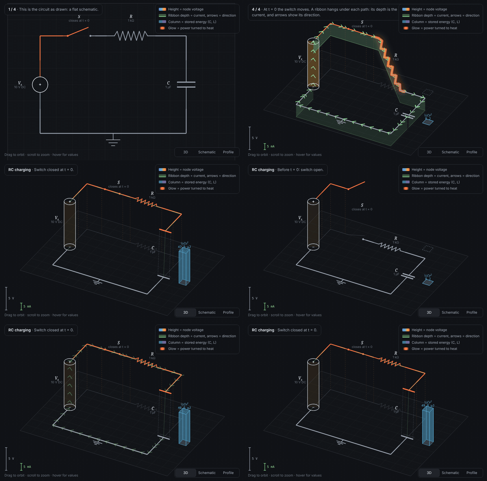
CircuitViz animation of an RC circuit charging, shown in 3D. Click to open the demo.
Click the animation to open the interactive demo →
CircuitViz, revisited demo

CircuitViz, revisited

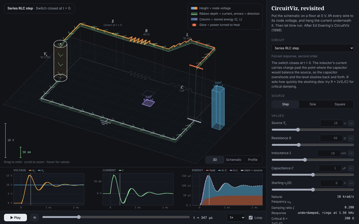
Put the schematic on a floor at 0 V, lift every wire to its node voltage, and hang the current underneath it as a ribbon — then let time run. Capacitors and inductors grow columns of stored energy, resistors glow with the power they turn into heat, and synchronized plots track voltage, current and energy. Six circuits: RC charging and discharging, RL energizing, the inductive kick, series RLC step and parallel RLC ringing.

Try:

  • Charge the RC circuit and watch the resistor burn exactly the energy the capacitor stores.
  • Open the switch in “RL inductive kick” and watch the node plunge below the floor.
  • Set the series RLC to R = 2√(L/C) for critical damping.

Based on E. R. Doering, “CircuitViz: a new method for visualizing the dynamic behavior of electric circuits,” IEEE Transactions on Education, vol. 39, no. 3, pp. 297–303, Aug. 1996 (doi:10.1109/13.538750). This version adds the energy columns, heat glow, energy bookkeeping, moving arrows, synchronized plots and the build-up animation.

Open the demo →
ECE380 — Discrete Time Signals and Systems

ECE380 course page →

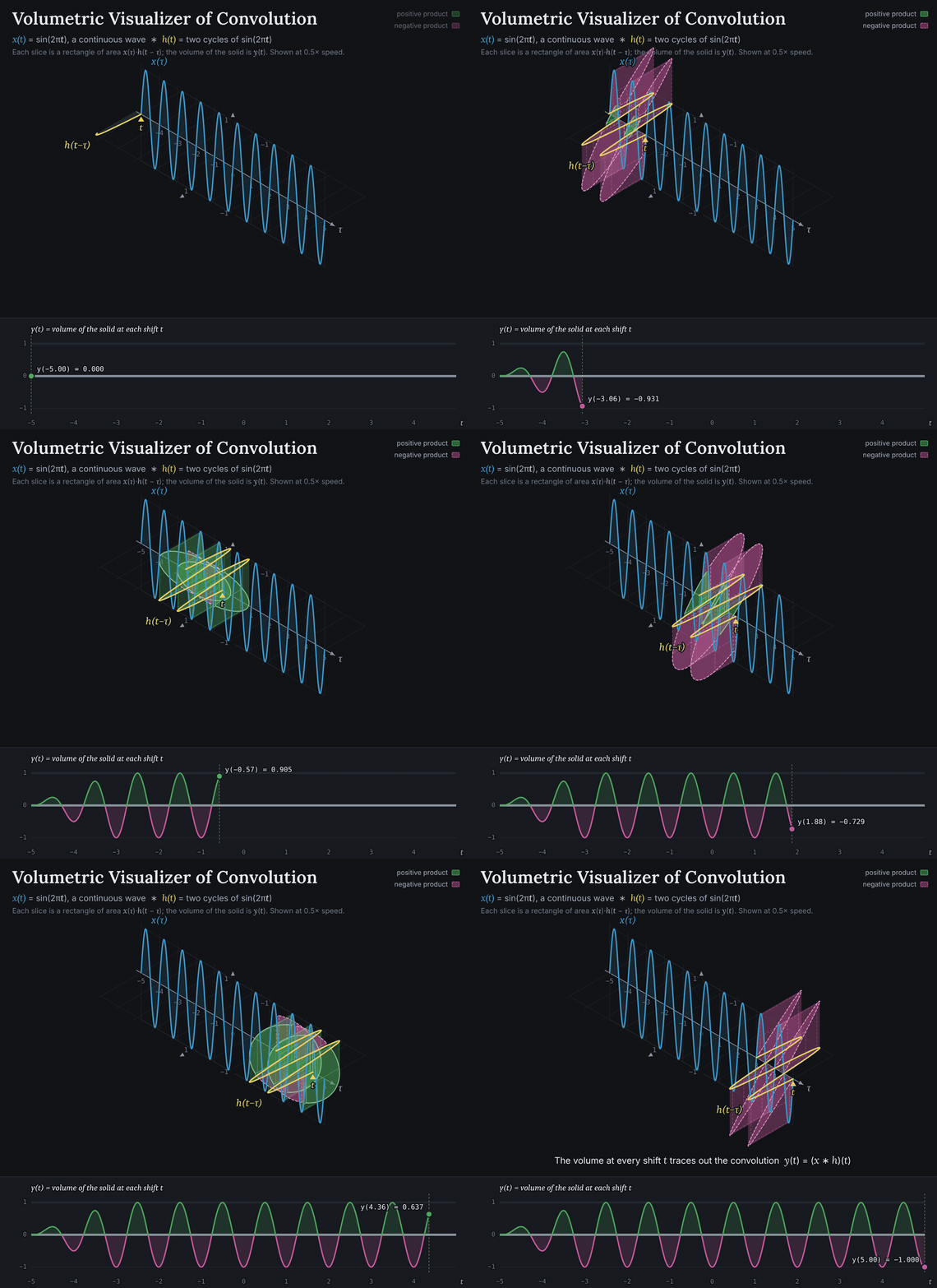
Volumetric visualizer of convolution. Click to open the interactive demo.
Click the animation to open the interactive demo →
Convolution as Volume demo

Convolution as Volume

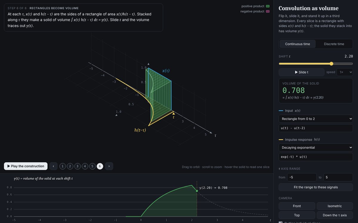
Convolution is usually taught as flip-and-slide, with the area under a product shaded. This demo adds a dimension: the flipped, shifted impulse response h(t−τ) is rotated out of the plane, so at every τ the product x(τ)·h(t−τ) is the area of a rectangle, and y(t) is the volume of the solid those rectangles stack into.

Try:

  • Convolve two rectangles and watch the volume trace out a triangle.
  • Use the “One sine cycle” input to see negative volume.
  • Switch to discrete time and check that the boxes add up to y[n].
Open the demo →
Bilinear Transform Warp demo

Bilinear Transform Warp

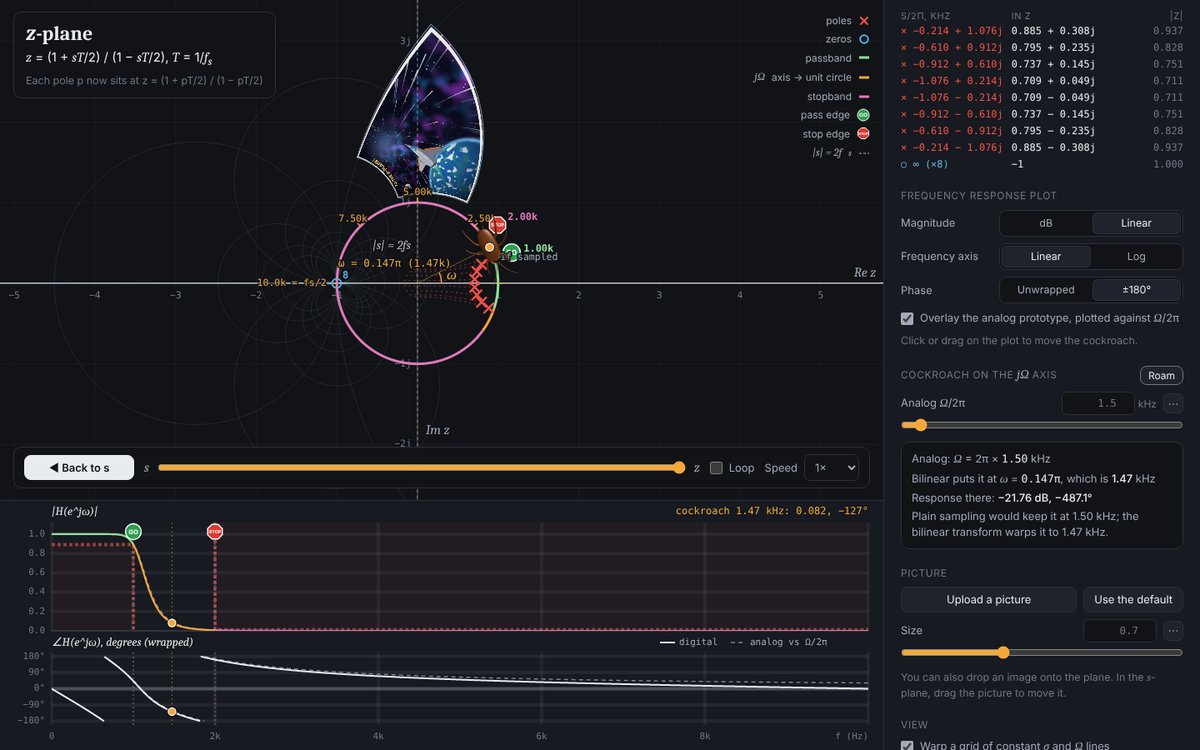
Watch the s-plane morph continuously into the z-plane under z = (1 + sT/2)/(1 − sT/2). Design a Butterworth or Chebyshev lowpass filter, see the edges prewarped, and follow each pole from the s-plane into the unit circle. A cockroach walking the jΩ axis shows where each analog frequency lands.

Try:

  • Lower the sample rate and watch the poles crowd toward z = 1.
  • Compare Butterworth and Chebyshev at the same specs.
  • Push the stop edge past Nyquist and read the aliasing warning.
Open the demo →
FIR Design by Windowing demo

FIR Design by Windowing

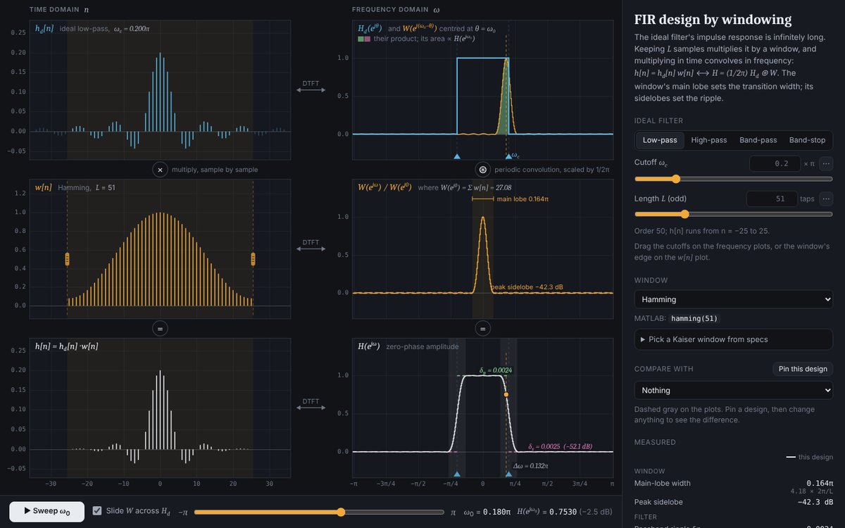
An ideal low-pass, high-pass, band-pass or band-stop impulse response is infinitely long, so an FIR filter keeps L samples of it through a window. Six linked plots show both sides at once: h_d[n] × w[n] = h[n] in time, and the brick wall convolved with the window’s spectrum in frequency. Pick from 11 MATLAB windows and copy h[n] into MATLAB or Python.

Try:

  • Lengthen the rectangular window: the transition narrows, but the ~9% Gibbs overshoot stays.
  • Switch Rectangular → Hamming → Blackman and watch attenuation trade against transition width.
  • Use “Pick a Kaiser window from specs” for 60 dB and Δω = 0.1π.
Open the demo →

ECE597 — Graphs and Signals

ECE597 course page →

Spectral Graph Theory Lab demo

Spectral Graph Theory Lab

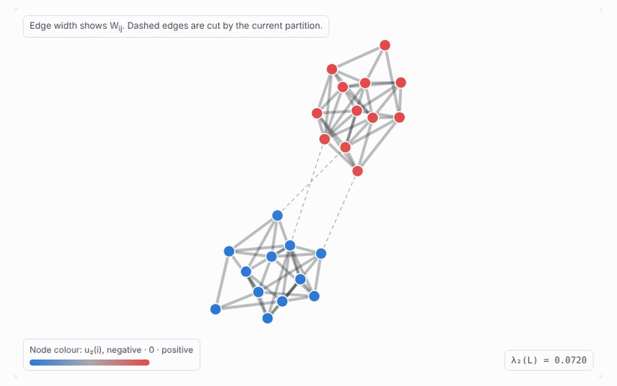
Change a graph continuously and watch its Laplacian spectrum respond. Connectivity, cuts, clusters and spanning trees can all be read from the eigenvalues — Fiedler vectors, Cheeger sweep cuts, spectral clustering and the matrix-tree theorem are each checked live as the graph morphs.

Open the demo →
Graph Fourier Explorer demo

Graph Fourier Explorer

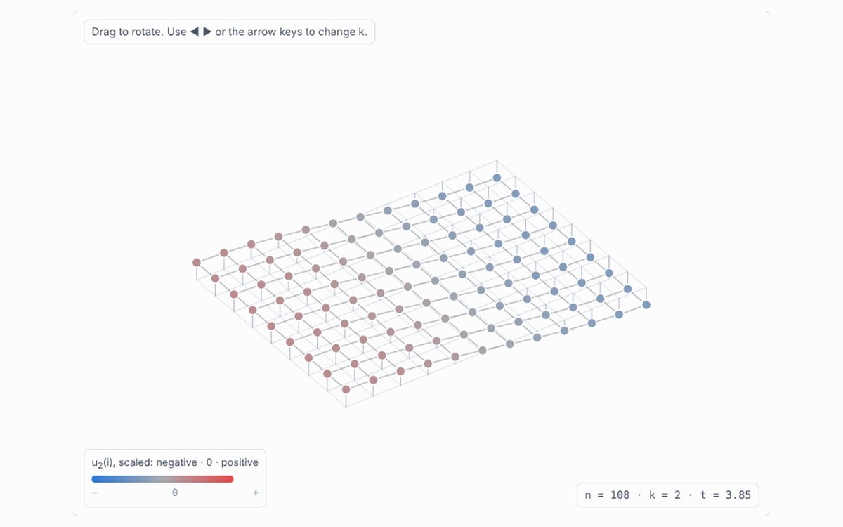
Eigenvectors of the graph Laplacian are the graph’s standing waves. Animate them in 3-D, watch heat and waves spread through their frequencies, and filter signals in the graph Fourier domain with low-pass, heat-kernel and Tikhonov filters.

Open the demo →
Graph Measures Explorer demo

Graph Measures Explorer

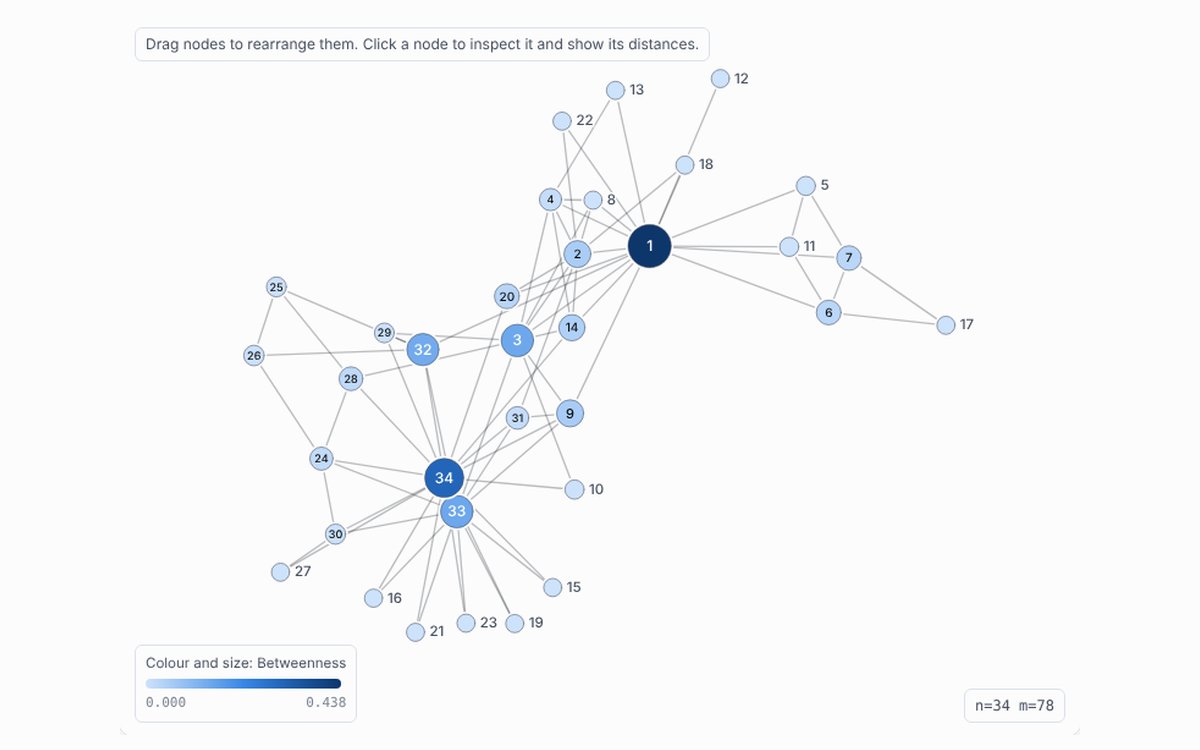
Centrality, clustering, cores and modularity on graphs you can generate or draw — including Zachary’s karate club. Every number on the page comes from the equation printed beside it, with normalisations matching NetworkX.

Open the demo →
Betti Numbers Explorer demo

Betti Numbers Explorer

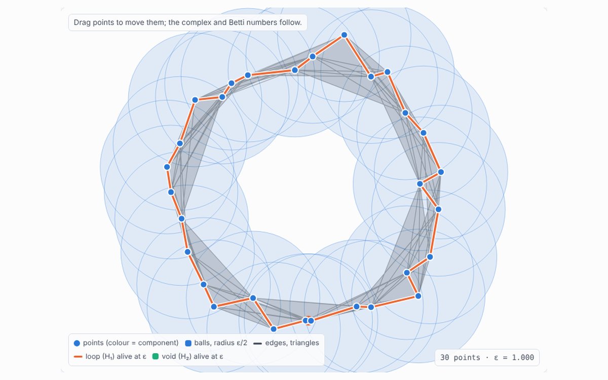
β₀ counts connected pieces, β₁ independent loops, β₂ enclosed voids. Grow Vietoris–Rips and Čech complexes from point clouds or build them by hand, read the persistence barcode, and see each Betti number computed from its boundary matrices.

Open the demo →